Data Exploration: $2.00 a Day
Introduction
This activity will introduce you to data on poverty in the U.S. We’ll begin with an overview of how poverty is measured in the U.S. and explore census data on poverty. The objectives of this exercise are to:
- state how poverty is defined
- discover poverty trends in your home state
Students will work in pairs to complete this assignment. One person should keep this instructions page open while the other navigates to Duke’s RStudio server. Record your answers on the hardcopy of this worksheet provided in class.
How is poverty defined and measured?

The U.S. Census Bureau (BOC) produces official estimates of poverty in America. The most famous data product of the BOC is the decennial population and housing census of the U.S., but the Bureau—part of the Department of Commerce—also conducts more than 130 annual surveys related to the population and economy. The BOC’s two main sources of data on poverty are the Current Population Survey Annual Social and Economic Supplement (CPS ASEC) and the American Community Survey. Go here to read about these two surveys.
The BOC produces an official and a supplemental estimate of poverty. Go here to read about the differences in each measure.
How is the federal poverty line (threshold) determined?
As they do every September, the BOC released new data and estimates from the CPS ASEC and ACS this week. You can now download and explore all of the 2016 data and data products. This is a demographer’s favorite week of the year by far. Check out the press releases for the new ACS and CPS ASEC.
Exploring poverty data
The BOC makes it easy to get started exploring data about income and poverty in the U.S. Just go to data.census.gov and search for data on “poverty”.
Platforms like this are nice for quick stat grabs, but often we need to work with the underlying data. Let’s give it a try in R. Start by navigating to https://vm-manage.oit.duke.edu/containers in your browser. You should be prompted to login with your NetID. Click on the link to “RStudio” to begin your R session.
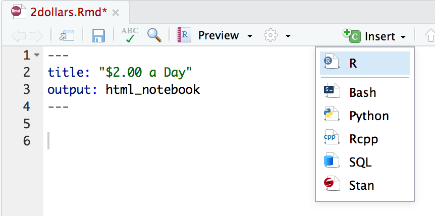
Click on “File” and choose “New File” and “R Notebook”. Change the title to “$2.00 a Day”.
Click “Preview”. You will be prompted to save the file. Make a new folder for this class and name the file “2dollars”. When you save, your browser might prompt you to allow pop-ups from RStudio.

Delete everything from line 6 down.
We’ll a few packages that will make exploration and mapping a breeze:
tidyverseandtidycensus. To install these packages, copy and run the following in your console (not the new file you created):
install.packages("tidyverse", dependencies=TRUE)
install.packages("purrr")
install.packages("tidycensus", dependencies=TRUE)
install.packages("leaflet")
install.packages("stringr")
install.packages("sf")- Wait for the code finish running. Then use the insert button to insert a new R code chunk.
- Next, load the packages (libraries) by typing the following inside your new chunk and hitting the play button.
# load packages
  library(tidyverse)
  library(tidycensus)
  library(leaflet)
  library(stringr)
library(sf)- Register for a BOC API key here.
- Check your email for the key. Copy the key and run the following code in your console (replacing “YOUR_KEY_HERE”)
census_api_key("YOUR_KEY_HERE", install=TRUE)- Create another new R chunk and paste in the following code to get the data on poverty in any state you choose. We’ll follow this example from Julia Silge.
  pop <- get_acs(geography = "county",
                 variables = "B01003_001",
                 state = "NC",
                 geometry = TRUE)

  pop
Just change the variable code (B17001_001) to explore a different variable in the ACS. Go here to see the options.
pal <- colorNumeric(palette = "viridis", domain = pop$estimate)

pov %>%
    st_transform(crs = "+init=epsg:4326") %>%
    leaflet(width = "100%") %>%
    addProviderTiles(provider = "CartoDB.Positron") %>%
    addPolygons(popup = ~ str_extract(NAME, "^([^,]*)"),
                stroke = FALSE,
                smoothFactor = 0,
                fillOpacity = 0.7,
                color = ~ pal(estimate)) %>%
    addLegend("bottomright",
              pal = pal,
              values = ~ estimate,
              title = "County Populations",
              opacity = 1)